Getting Started with torchxai

torchxai is a PyTorch explainability library with a one-line API: explain(model, image). It works with CNNs (ResNet, VGG, EfficientNet) and Vision Transformers (ViT, DeiT, Swin), and accepts images in virtually any format.

---

Table of Contents

1. Installation
2. Your First Explanation in 60 Seconds
3. All Input Types
4. Choosing a Method
5. Using Individual Explainers
6. Saving and Exporting
7. Next Steps

---

Installation

From PyPI (recommended)

pip install torchxai-explain

Note: The PyPI package is torchxai-explain, not torchxai. Installing torchxai will give you a different, unrelated package.

From Source

git clone https://github.com/torchxai/torchxai.git
cd torchxai
pip install -e .

Verify Your Installation

python -c "import torchxai; print('OK')"

Expected output:

OK

Requirements

• Python 3.8 or later
• PyTorch 1.10 or later
• torchvision

If you have a GPU, torchxai will use it automatically when your model is on a CUDA device. No extra steps required.

---

Your First Explanation in 60 Seconds

The following complete example loads a pretrained ResNet-50, runs it on an image, and produces a visual explanation of which pixels drove the prediction.

import torch
import torchvision.models as models
from torchxai import explain, show_explanation

# 1. Load a pretrained model and put it in eval mode
model = models.resnet50(weights="IMAGENET1K_V1")
model.eval()

# 2. Point to your image — a file path string works out of the box
image = "path/to/your/image.jpg"

# 3. Generate the explanation with a single call
explanation = explain(model, image)

# 4. Visualize it
show_explanation(explanation)

That's it. explain() handles preprocessing, forward/backward passes, and heatmap generation automatically.

The output looks like this — a heatmap overlaid on the original image, highlighting the regions the model found most important:

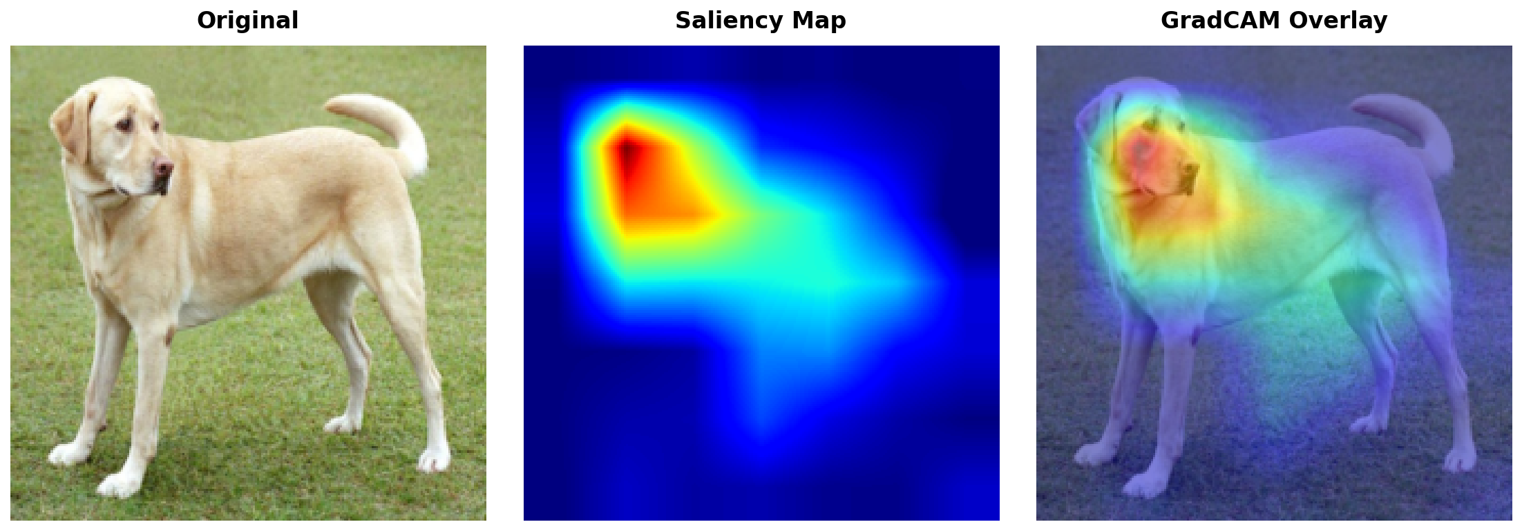
Warmer colors (red/yellow) indicate regions with high importance; cooler colors (blue) indicate low importance.

---

All Input Types

torchxai accepts images in five formats. Use whichever is most natural for your workflow.

1. File Path String

The simplest option when you have an image on disk.

from torchxai import explain

explanation = explain(model, "path/to/image.jpg")

2. pathlib.Path

Works identically to a string path. Useful when your paths are already Path objects.

from pathlib import Path
from torchxai import explain

image_path = Path("path/to/image.jpg")
explanation = explain(model, image_path)

3. PIL Image

Use this when you have already loaded or processed an image with Pillow.

from PIL import Image
from torchxai import explain

pil_image = Image.open("path/to/image.jpg").convert("RGB")
explanation = explain(model, pil_image)

4. NumPy Array

Use this when your image comes from OpenCV, scikit-image, or any other NumPy-based pipeline.

import numpy as np
from torchxai import explain

# Shape: (H, W, C), dtype: uint8 or float32
numpy_image = np.array(Image.open("path/to/image.jpg"))
explanation = explain(model, numpy_image)

5. PyTorch Tensor

Use this when you are already working in PyTorch — for example, pulling a batch from a DataLoader.

import torch
from torchxai import explain

# 4D batch tensor: (1, C, H, W)
batch_tensor = torch.randn(1, 3, 224, 224)
explanation = explain(model, batch_tensor)

# 3D single-image tensor: (C, H, W) — also accepted
single_tensor = torch.randn(3, 224, 224)
explanation = explain(model, single_tensor)

Tip: When passing tensors, torchxai assumes your values are already preprocessed (normalized to ImageNet statistics). If you pass a raw tensor with pixel values in [0, 255], the model may produce poor predictions. See Common Mistakes for details.

---

Choosing a Method

torchxai supports six explanation methods. The default (used when you call explain(model, image)) is GradCAM.

Method Comparison

Method	Works With	Speed	Heatmap Quality	Requires Gradients	Best For
gradcam	CNNs	Fast	High	Yes	General CNN explanations
eigencam	CNNs	Very fast	Medium	No	Large batches, fast iteration
layercam	CNNs	Fast	High (fine-grained)	Yes	Detailed spatial explanations
gradcam++	CNNs	Fast	High	Yes	Multiple objects in scene
attention_rollout	ViTs	Fast	High	No	Vision Transformers
transformer_attribution	ViTs	Medium	Very high	Yes	High-quality ViT explanations

Specifying a Method

Pass the method argument to explain():

from torchxai import explain

# Use GradCAM (default)
explanation = explain(model, image, method="gradcam")

# Use EigenCAM for faster results
explanation = explain(model, image, method="eigencam")

# Use AttentionRollout for a Vision Transformer
explanation = explain(vit_model, image, method="attention_rollout")

Quick Recommendations

• Unsure where to start? Use gradcam. It works well on virtually all CNN architectures with no tuning.
• Working with a Vision Transformer (ViT, DeiT, Swin)? Use attention_rollout. It is fast and leverages the model's native attention mechanism.
• Need the highest quality ViT explanation? Use transformer_attribution. It takes a little longer but produces sharper, more faithful heatmaps.
• Need the fastest possible results (large batches, real-time pipelines)? Use eigencam. It requires no gradient computation.
• Detecting multiple objects? Use gradcam++. It handles multi-instance scenes better than standard GradCAM.
• Need fine-grained spatial detail? Use layercam. It produces higher-resolution activations than GradCAM.

---

Using Individual Explainers

In addition to the explain() shortcut, you can instantiate explainer classes directly. This is useful when you want to reuse the same explainer across many images without re-initializing it each time.

GradCAM

import torchvision.models as models
from torchxai import GradCAM, show_explanation

model = models.resnet50(weights="IMAGENET1K_V1")
model.eval()

# Instantiate once
explainer = GradCAM(model)

# Reuse for many images
explanation1 = explainer.explain("image1.jpg")
explanation2 = explainer.explain("image2.jpg")

show_explanation(explanation1)

EigenCAM

from torchxai import EigenCAM

explainer = EigenCAM(model)
explanation = explainer.explain("image.jpg")

LayerCAM

from torchxai import LayerCAM

explainer = LayerCAM(model)
explanation = explainer.explain("image.jpg")

GradCAM++

from torchxai import GradCAMPlusPlus

explainer = GradCAMPlusPlus(model)
explanation = explainer.explain("image.jpg")

AttentionRollout (Vision Transformers)

import torchvision.models as models
from torchxai import AttentionRollout, show_explanation

# Load a Vision Transformer
vit_model = models.vit_b_16(weights="IMAGENET1K_V1")
vit_model.eval()

explainer = AttentionRollout(vit_model)
explanation = explainer.explain("image.jpg")

show_explanation(explanation)

TransformerAttribution (Vision Transformers)

from torchxai import TransformerAttribution

explainer = TransformerAttribution(vit_model)
explanation = explainer.explain("image.jpg")

Targeting a Specific Layer

By default, torchxai targets the last convolutional (or attention) layer. You can override this:

from torchxai import GradCAM

# Specify any named layer in your model
explainer = GradCAM(model, target_layer="layer3")
explanation = explainer.explain("image.jpg")

To find the valid layer names for your model:

for name, module in model.named_modules():
    print(name)

---

Saving and Exporting

Display in a Window or Notebook

show_explanation() renders the heatmap overlaid on the original image. In a Jupyter notebook it displays inline; in a script it opens a window.

from torchxai import explain, show_explanation

explanation = explain(model, "image.jpg")
show_explanation(explanation)

Save a Heatmap to Disk

save_heatmap() writes the raw heatmap (without overlay) to a file.

from torchxai import explain, save_heatmap

explanation = explain(model, "image.jpg")
save_heatmap(explanation, save_path="outputs/heatmap.png")

Overlay a Heatmap on the Original Image

overlay_heatmap() returns a blended image with the heatmap superimposed on the original. You can then save or display it.

from torchxai import explain, overlay_heatmap
from PIL import Image

explanation = explain(model, "image.jpg")

# Returns a PIL Image with the overlay applied
overlaid = overlay_heatmap(explanation, alpha=0.5)
overlaid.save("outputs/overlaid.png")

The alpha parameter controls opacity: 0.0 shows only the original image, 1.0 shows only the heatmap.

Create a Side-by-Side Comparison

create_comparison() produces a single image with the original and the explanation side by side — useful for reports and presentations.

from torchxai import explain, create_comparison

explanation = explain(model, "image.jpg")

# Saves a side-by-side PNG and also returns it as a PIL Image
comparison = create_comparison(explanation, save_path="outputs/comparison.png")

Complete Export Workflow

import torchvision.models as models
from torchxai import explain, show_explanation, save_heatmap, overlay_heatmap, create_comparison

model = models.resnet50(weights="IMAGENET1K_V1")
model.eval()

explanation = explain(model, "image.jpg")

# Display interactively
show_explanation(explanation)

# Save raw heatmap
save_heatmap(explanation, save_path="outputs/heatmap.png")

# Save overlaid image
overlaid = overlay_heatmap(explanation, alpha=0.5)
overlaid.save("outputs/overlaid.png")

# Save side-by-side comparison
create_comparison(explanation, save_path="outputs/comparison.png")

---

Next Steps

• API Reference — full documentation for every function and class, including all parameters and return types.
• Methods — deep-dive into how each explanation method works, with mathematical background and guidance on when to use each.
• Advanced Usage — custom preprocessing, batched explanations, integrating with training loops, and more.
• Troubleshooting — solutions to common errors and frequently asked questions.